Index-Match-Match: How to Index-Match Rows and Columns

In many cases, Excel data can be easily merged with a single INDEX-MATCH (or a VLOOKUP). Sometimes, though, it's time to bring out the big guns—the INDEX-MATCH-MATCH.

INDEX-MATCH-MATCH combines two MATCH statements into the row and column positions in an INDEX formula. In doing so, you're making a fillable formula left, right, up, or down for when you merge or find data.

In this step-by-step guide, we'll create an INDEX-MATCH formula and then add the second MATCH statement to make it an INDEX-MATCH-MATCH.

How Merging Data in Excel Works

There are two main ways to merge data in Excel — VLOOKUP and INDEX-MATCH. They work similarly. 

With both VLOOKUP and INDEX-MATCH, you have a search term that you want to find in a column. When Excel finds the search term, it looks for the corresponding value on the same row in another column. It's like finding a phone number in a phone book.

If you've never held a phone book, here's an image below for reference. (Did you know the last phone books were published in 2010?) Back in the olden days, you would open the phone book, flip through the pages to find a last name or business, and then move your finger over one or two columns to find the phone number. VLOOKUP and INDEX-MATCH do the exact same thing.

Ultimately, you're trying to programmatically find information you don't know with information you do know. That's the idea of merging data. VLOOKUP and INDEX-MATCH do have some differences, however. 

The Difference Between VLOOKUP and INDEX-MATCH

With both, you tell Excel to find a value on a row and then return it in a column beside it. There are a couple of differences, though.

• Indexing Directions: The biggest difference is that VLOOKUP only looks right. A VLOOKUP array includes the lookup_array as well as the array. In other words, you have to initially select both the search and output columns. The selection starts with the search column, and VLOOKUP only looks to the right of that. INDEX-MATCH can look both left and right.

• Referencing Adjacent Cells: When writing a VLOOKUP formula, you must manually enter the number of columns from the search column.

• Multiple columns: Unlike VLOOKUP, INDEX-MATCH can index multiple columns for fillable output. In other words, the array can be multiple columns. When properly using referencing, you can pull a formula across a sheet and fill multiple columns.

When to Use INDEX-MATCH

Like any data merge, INDEX-MATCH works best when you have a common, unique identifier between two data sources. INDEX-MATCH is best for merging data with unique identifiers, including:

• Customer IDs

• SKUs

• URLs

• States or zip codes

These are examples of primary keys. For a quick merge, the common value doesn't have to be as stringent as required for a primary key, but it should, at the very least, be unique. If there are duplicates in your search array, INDEX-MATCH returns the value from the first instance, which might not be accurate.

Parts of the INDEX-MATCH and INDEX-MATCH-MATCH

To accomplish an INDEX-MATCH-MATCH, you'll need a few parts.

Worksheet

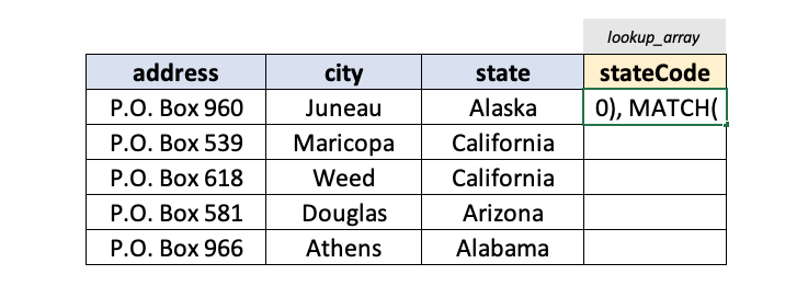
The worksheet is your working document or section of a worksheet. In our example, we'll use a short list of addresses. Note the stateCode column. That's where we'll write the INDEX-MATCH-MATCH formula.

NOTE: In many cases, you'll work on a different worksheet than the output array. We won't do that in this example. Everything will be on one sheet.

Search Array

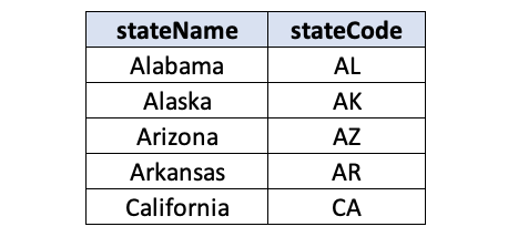
This is like the answer key. It contains the list of values you'll be searching for and the answer you want. In this case, it'll be a list of states and their state codes. But the search array can be much, much bigger.

To put these two sheets into context, here's our goal outcome.

• Absolute referencing: In this example, we'll be using absolute and relative referencing. Colloquially, these equate to "locking" selections on a particular set of cells, column, or row. Here's a quick key for referencing:

• Absolute row, absolute column ($A$1:$B$2). This will lock your search on these cells. We'll lock both the rows and columns when referencing the search array.

• Absolute column, relative row ($A1:$A20). This will lock the column but not the row. This will be useful when we write the first MATCH formula.

• Absolute row, relative column (A$1). This will lock the row but not the column. This will be useful when we write the second MATCH formula.

The INDEX-MATCH-MATCH formula

The formula we're using has three parts.

Here's how the formula breaks down:

• FORMULA = INDEX(array, row_num, [col_num])

  • array: A list of values that live to the left or right of the search value (ex. stateCode).

  • row_num / col_num: Index typically operates on cell coordinates (ex. 2, 2). We'll replace these with MATCH statements.

• MATCH(lookup_value, lookup_arraymore extensivech_type])

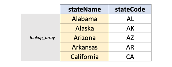
  • lookup_array: A list of values you want to search against (ex. state column).

  • lookup_value: The thing you want to find the search array (ex. state cell).

  • match_type: How you want to match. We'll use "0" for an exact match.

In this case, we have the "state list" and the "address list". The state list is a list of states and their state codes. The other part is the address list. We'll reference the state list from the address list with the INDEX-MATCH.

Step 1: Create an Output Column

In your worksheet, create a column and label it the same as the output array. It's best to either copy and paste or reference the cells to make sure they're exactly the same. That'll be important later.

Step 2: Start Writing the Formula in the stateCodeColumn

We'll start writing our formula in the first cell of the new column. If we've done our referencing properly, we'll be able to fill the cell down later.

Step 3: Tell Excel Where You Want to Search

Remember that the state list maps states' names to their abbreviations. It's like the answer key. The array is the list of values you want in your new stateCode column.

We'll want to lock that entire selection because it should never change, so we'll use absolute referencing. If this selection were relative, when we index down the new stateCode column, the array would move, too, and start mapping Alabama to AK, then AZ, then AR… We don't want that. Absolute referencing is important.

FORMULA = INDEX($B$1:$B$5, MATCH(lookup_value, lookup_array, [match_type]),)

Step 4: Tell Excel What You Want to Find

FORMULA = INDEX($B$1:$B$5, MATCH($C1, lookup_array, [match_type]),)

Excel now knows what you want in your cell. Now you have to tell it what you want as your reference point. That's the lookup_value of the nested MATCH formula.

Note the absolute column. By locking the column, you can drag this formula right, up, or down without losing the referencing, which will be important later.

Step 5: Tell Excel Where You Want to Search

You have your search term. Now tell Excel where to look for it. In this case, it'll be the state list—your answer key.

FORMULA = INDEX($B$1:$B$5, MATCH($C1, $A$1:$A$5, [match_type]),)

Step 6: Tell Excel How You Want to Search

FORMULA = INDEX($B$1:$B$5, MATCH($C1, $A$1:$A$5, 0),)

The match_type value has three positions: -1, 0 and 1

The match_type function is not case-sensitive and also takes wildcard characters (*). You'll know if you did something wrong if the function returns #N/A.

In this case, we'll use the exact match function because state names are discrete.

Step 7: The Second MATCH

While INDEX-MATCH relies on row coordinates to index columns, INDEX-MATCH-MATCH also needs a column for reference. You'll remember that INDEX-MATCH works best with unique identifiers. INDEX-MATCH-MATCH is no different. Make sure your column headers are unique. Otherwise, Excel will only reference the first column header.

In this step, we'll start the second MATCH statement. It's exactly the same as the first MATCH statement, but referencing the column.

In the first MATCH, we locked the column with absolute referencing ($C1). In the second MATCH, we lock the row (D$1) so the formula won't move down with the formula. Instead, it'll move across the columns.

FORMULA = INDEX($B$1:$B$5, MATCH($C1, $A$1:$A$5, 0), MATCH(D$1, lookup_array, [match_type]))

Step 8: Map the Columns to the Dataset Columns

Just like the first MATCH, we'll need to tell the formula where to find the search term. In the second MATCH, it'll be the column cell (or cells).

FORMULA = INDEX($B$1:$B$5, MATCH($C1, $A$1:$A$5, 0), MATCH(D$1, $B$8, [match_type]))

Step 9: Tell Excel How to Match Again

Just like the first MATCH statement, we'll use the exact match — 0. We want to find exactly the right column to make this formula bulletproof. It might not make sense now, but the next steps will show how this applies to enormous datasets.

FORMULA = INDEX($B$1:$B$5, MATCH($C1, $A$1:$A$5, 0), MATCH(A$1, $B$2, 0))

Step 10: See What Happens

Hit enter to commit the formula, and you should see AK in the first cell.

Here's a diagram of what happened in the first MATCH statement:

1. Excel knows to look for the lookup_value "Alaska" in the lookup_array.

2. The formula finds "Alaska" in the lookup_array.

3. The formula follows the row over to the array, or the stateCode column.

4. The formula returns the value to the output cell.

Step 11: Fill Your Formula Down

There are several ways to fill a column down. Pick the one that feels the most comfortable. Hotkeys are the fastest, but the others will do the job, too.

• Double-click: Double-click the square in the bottom-right corner of the cell.

• Hotkeys: Select down with CTRL + down arrow, then fill down with CTRL + D.

• Drag and pull: Drag the bottom-right corner down the column.

• Copy and paste: With properly referenced Excel formulas, you can just copy and paste into a new cell, and the formula will move with it.

Congrats! You've completed an INDEX-MATCH-MATCH.

When to Use the INDEX-MATCH-MATCH

The INDEX-MATCH is an invaluable formula for merging data. The INDEX-MATCH-MATCH allows you to also match column headers. It's really useful for paring down large datasets into manageable ones.

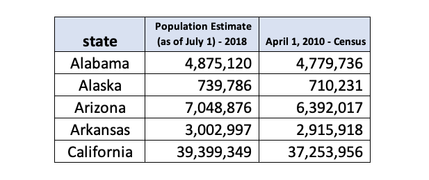
For instance, let's say you have 11 columns and 51 rows of U.S. Census data.

You could easily compile data for five consecutive states manually. The dataset isn't huge. But imagine you had 100 columns and 50,000 rows of customer, advertising, or inventory data. That's a job for INDEX-MATCH-MATCH.

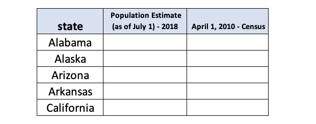
In this scenario, we want to pull select U.S. Census data into a friendlier format. Instead of hunting through the spreadsheet, we can simply copy and paste (or reference) the headers to this new sheet. We'll use two non-adjacent, non-consecutive columns to illustrate how this works.

If you've built the formula correctly, then you can just fill right from the stateCode column to populate the rest of the spreadsheet. With INDEX-MATCH-MATCH, it doesn't matter whether the columns or even the lookup terms are in the same order as the sheet.

When properly referenced, the INDEX-MATCH-MATCH does a great job of returning the data you want from a big dataset or merging data.

Learn More with Excel Training from CBT Nuggets

Formulas are useful for slicing and parsing data in Excel, but some great features are baked into the software, too. For instance, you could just as easily create a pivot table or use filtering to do the same thing. CBT Nuggets trainer Simona Millham has training for every skill level, from basic to advanced.

Start learning Excel today!